Pull/push distributions

In this example, we show how to use moscot.plotting.push() and moscot.plotting.pull() plotting functions.

Note

These visualization functions are only implemented for non-spatial problems.

To see how pull-back or push-forward cell distributions can be visualized for problems incorporating spatial information, please have a look at the Tutorials. Here, we use the hspc() dataset to demonstrate the usage of moscot.plotting.push() and moscot.plotting.pull() with the TemporalProblem. In this context, the pull-back distribution corresponds to the set of ancestor cells, while the push-forward distribution corresponds to the set of descending cells.

See also

• See Cell transitions on how to plot cell transitions.

• See Sankey diagram on how to plot the Sankey diagram.

Imports and data loading

import warnings

warnings.simplefilter("ignore", UserWarning)
warnings.simplefilter("ignore", FutureWarning)

import moscot.plotting as mtp
from moscot import datasets
from moscot.problems.time import TemporalProblem

Load the hspc() dataset.

adata = datasets.hspc()
adata

AnnData object with n_obs × n_vars = 4000 × 2000
    obs: 'day', 'donor', 'cell_type', 'technology', 'n_genes'
    var: 'n_cells', 'highly_variable', 'means', 'dispersions', 'dispersions_norm'
    uns: 'cell_type_colors', 'hvg', 'neighbors', 'neighbors_atac', 'pca', 'umap'
    obsm: 'X_lsi', 'X_pca', 'X_umap_ATAC', 'X_umap_GEX', 'peaks_tfidf'
    varm: 'PCs'
    obsp: 'connectivities', 'distances', 'neighbors_atac_connectivities', 'neighbors_atac_distances'

Prepare and solve the problem

First, we need to prepare and solve the problem. Here, we set the threshold parameter to a relatively high value to speed up convergence at the cost of a lower quality solution.

tp = TemporalProblem(adata).prepare(time_key="day").solve(epsilon=1e-2, threshold=1e-2)

INFO     Ordering Index(['4c45fb900fbb', 'c462df3e03b5', '27b9aa554758', '9a0cbad09594',                           
                '98b88fc30c58', '5008d863224a', '904d6bcfd520', '5287a74337a0',                                    
                '862d6d6e4e49', '288e38fb37aa',                                                                    
                ...                                                                                                
                '038518e366a9', '809ba84a9cbb', '4264c55de7d0', 'a7097007fbea',                                    
                '1381ec6cb466', '946cf349f84e', 'da6baa1b0624', 'ba7d40e15f3d',                                    
                '69451694ec4c', '193992d571a5'],                                                                   
               dtype='object', name='cell_id', length=4000) in ascending order.                                    
INFO     Computing pca with `n_comps=30` for `xy` using `adata.X`                                                  

INFO     Computing pca with `n_comps=30` for `xy` using `adata.X`                                                  
INFO     Computing pca with `n_comps=30` for `xy` using `adata.X`                                                  
INFO     Solving `3` problems                                                                                      
INFO     Solving problem BirthDeathProblem[stage='prepared', shape=(766, 1235)].                                   

No GPU/TPU found, falling back to CPU. (Set TF_CPP_MIN_LOG_LEVEL=0 and rerun for more info.)

INFO     Solving problem BirthDeathProblem[stage='prepared', shape=(1235, 1201)].                                  
INFO     Solving problem BirthDeathProblem[stage='prepared', shape=(1201, 798)].                                   

As for all plotting functionalities in moscot, we first call the method of the problem class, which stores the results of the computation in the AnnData instance. Let us assume we look for the descendants of cells of time point 4 in time point 7. We can specify whether we want to return the result via the return_data parameter.

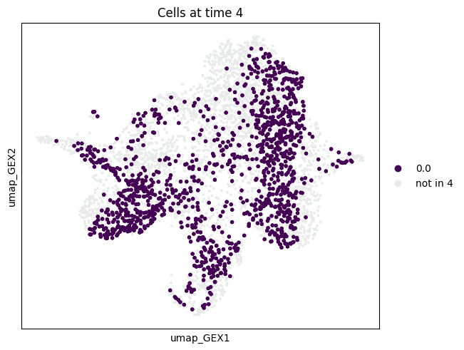
tp.push(source=4, target=7)

Plot push distribution

We can now visualize the result. As we have multiple time points in the UMAP embedding, it is best to visualize in one plot all the cells corresponding to time point 4, and then the ones corresponding to the descending cells. As the AnnData instance contains UMAP embeddings for both gene expression and ATAC, we need to define which one to use via the basis parameter.

mtp.push(tp, time_points=[4], basis="umap_GEX")
mtp.push(tp, time_points=[7], basis="umap_GEX")

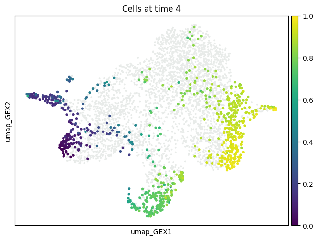
By default, the result of the TemporalProblem.push is saved in adata.uns['moscot_results']['push']['push'] and overrides this element every time the method is called. To prevent this, we can specify the parameter key_added, as shown below.

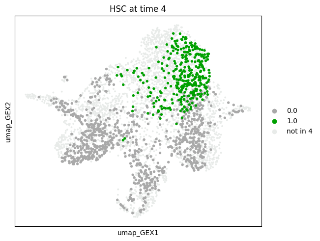
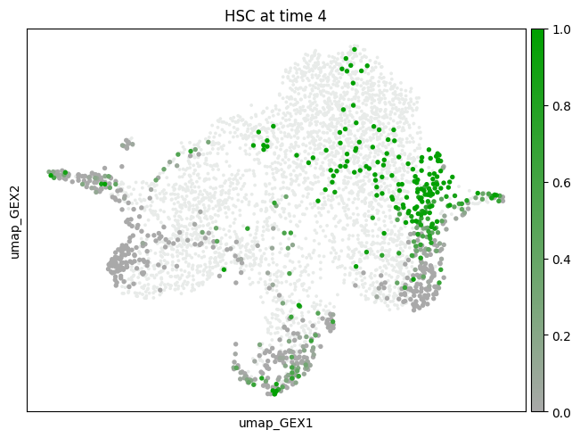
We can also visualize the descendants of only a subset of categories of an obs column by specifying the data and the subset parameter.

new_key = "subset_push"
tp.push(
    source=4,
    target=7,
    data="cell_type",
    subset="HSC",
    key_added=new_key,
)
mtp.push(tp, time_points=[4], key=new_key, basis="umap_GEX")
mtp.push(tp, time_points=[7], key=new_key, basis="umap_GEX")