Mapping gene expression in space
This tutorial shows how to use the MappingProblem for transferring gene expression from single-cell data to spatial data.
Mapping single-cell atlases to spatial transcriptomics data is a crucial analysis step to integrate cell type annotation across technologies. Furthermore, it is often the case that imaging-based spatial transcriptomics technologies only measure a limited set of transcripts, which could nonetheless be used as anchor features to map the gene expression of unobserved genes from single-cell data.
Note
For this tutorial, Squidpy is needed for spatial data plotting. You can either install it with:
pip install squidpyorpip install moscot[spatial]as an optional dependency ofmoscot
See also
If spatial coordinates are available for multiple datasets, see Alignment of spatial transcriptomics data on how to align spatial transcriptomics data, integrating both gene expression and spatial similarity.
Preliminaries
import warnings

import moscot as mt
from moscot import datasets
from moscot.problems.space import MappingProblem

import seaborn as sns

import scanpy as sc
import squidpy as sq

warnings.simplefilter("ignore", FutureWarning)
Dataset description
we will use a preprocessed and normalized dataset of the Drosophila embryo, originally used in NovoSpaRc [Nitzan et al., 2019]. In fact, the MappingProblem is essentially a reimplementation of the original Gromov-Wasserstein formulation from NovoSpaRc, yet with some technical innovations that make it more scalable.
Load the drosophila() dataset:
adata_sc = datasets.drosophila(spatial=False)
adata_sp = datasets.drosophila(spatial=True)
adata_sc, adata_sp
(AnnData object with n_obs × n_vars = 1297 × 2000
     obs: 'n_counts'
     var: 'n_counts', 'highly_variable', 'highly_variable_rank', 'means', 'variances', 'variances_norm'
     uns: 'hvg', 'log1p', 'pca'
     obsm: 'X_pca'
     varm: 'PCs'
     layers: 'counts',
 AnnData object with n_obs × n_vars = 3039 × 82
     obs: 'n_counts'
     var: 'n_counts'
     uns: 'log1p', 'pca'
     obsm: 'X_pca', 'spatial'
     varm: 'PCs'
     layers: 'counts')
Visualise the data
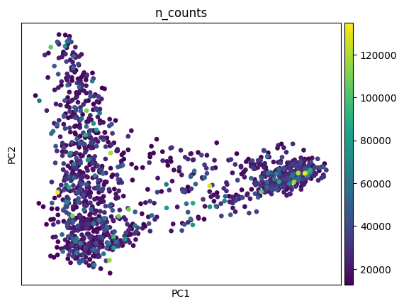
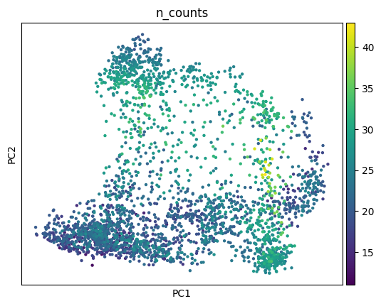
Let’s take a look at the data by plotting the number of counts first.
sc.pl.pca(adata_sc, color="n_counts")
sc.pl.pca(adata_sp, color="n_counts")
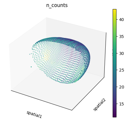
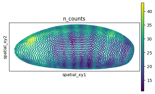
We can also visualize the spatial dataset in spatial coordinates. Here, it’s important to consider that the spatial dataset actually consists of measurements in 3D. We can visualize them with scanpy.pl.embedding() specifying projection="3d", as well as with squidpy.pl.spatial_scatter() after extracting only the \(x\), \(y\) coordinates.
sc.pl.embedding(
    adata_sp,
    basis="spatial",
    color="n_counts",
    projection="3d",
    na_color=(1, 1, 1, 0),
)

adata_sp.obsm["spatial_xy"] = adata_sp.obsm["spatial"][:, [0, 2]]
sq.pl.spatial_scatter(
    adata_sp,
    spatial_key="spatial_xy",
    color="n_counts",
    shape=None,
    size=20,
    figsize=(5, 3),
)
WARNING: Please specify a valid `library_id` or set it permanently in `adata.uns['spatial']`
Mapping single-cell gene expression in space
With moscot, it is possible to learn a single-cell-to-spatial mapping by leveraging fused Gromov-Wasserstein (FGW) optimal transport [Vayer et al., 2018]. A basic description of the algorithm is the following:
Given a set of observations that share some features in the metric space, and have some other features in different metric spaces, the FGW method aims at finding the optimal matching between these two set of observations, based both on shared and unique features. In our case:
the “shared” metric space could be the one defined by a set of genes that were measured in both single-cell and spatial transcriptomics data.
the “unique” metric spaces are the genes only measured in single-cell data and the spatial coordinates for the spatial transcriptomics data.
Prepare the MappingProblem
The moscot MappingProblem interfaces the FGW algorithm in a user-friendly API. First, let’s initialize the MappingProblem by passing the single-cell and spatial AnnData objects.
mp = MappingProblem(adata_sc=adata_sc, adata_sp=adata_sp)
After initialization, we need to prepare() the problem. In this particular case, we need to pay attention to 3 parameters:
sc_attr: specify the attribute inAnnDatathat we want to use for the features (genes) in the unique space. Usually, it’s theXattribute, which contains normalized counts, but a pre-computed PCA could also be used. Furthermore, for theuniquefeatures it might be desirable to use some other type of modality, for instance protein expression or ATAC-seq measurements, that could be stored for example inobsm.var_names: specify the set of genes that we desire to be using for thesharedspace, that is the common set of genes in both dataset. If set toNone, it will try to compute the intersection between the single-cell and spatial gene names.joint_attr: it is possible to also specify some other attributes that might be used for the “shared” features space, for instance, an embedding such as PCA.
If the number of shared features is large enough, it is also possible to compute a PCA on the “shared” gene space (by passing the xy_callback). We advise this if we are in the settings of \(>50\) genes shared between the two datasets.
Please see Passing callbacks in prepare() on how to use different callbacks.
mp = mp.prepare(sc_attr={"attr": "obsm", "key": "X_pca"}, xy_callback="local-pca")
INFO Preparing a :term:`quadratic problem`.
INFO     Computing pca with `n_comps=30` for `xy` using `adata.X`
INFO     Normalizing spatial coordinates of `x`.
Solve the MappingProblem
We are now ready to solve() the problem. The most important parameter to take into account is the alpha value, which balances the weight of each loss (“unique” vs. “shared” spaces). With alpha close to \(0\), the “shared” space loss is weighted more, with alpha close to \(1\), the “unique” space loss is weighted more. For the purpose of this example, we’ll use alpha=0.5 but we suggest to increase it if only a few features are present. It should take maximum one minute on a laptop.
mp = mp.solve()
INFO     Solving `1` problems
INFO     Solving problem OTProblem[stage='prepared', shape=(3039, 1297)].
Analysis of the transport plan
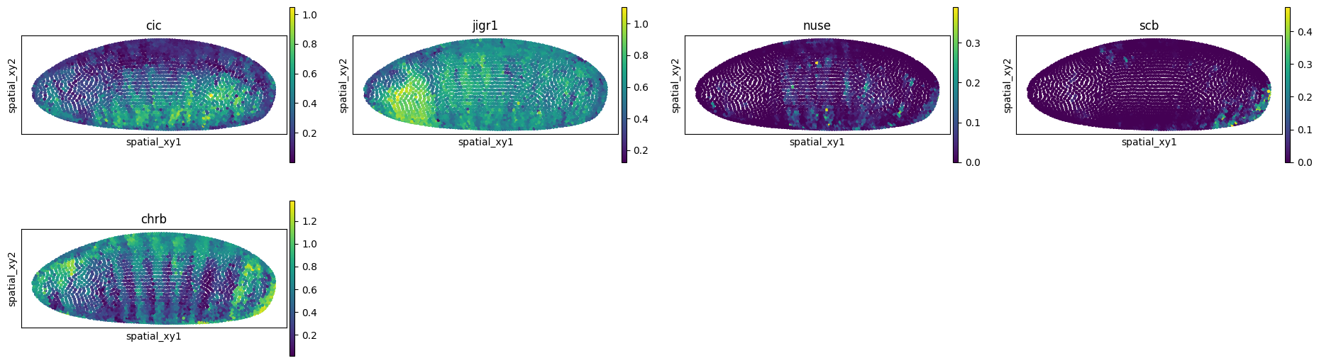
The first thing we might be interested in doing is “imputing” genes that were not present in the spatial data. We can do so by using the impute() method. For the purpose of the tutorial, we will select a few genes from the single-cell data.
If you are working on a GPU with large data, you might want to pass device='cpu' to the method in order to use the CPU memory for this task.
genes = ["cic", "jigr1", "nuse", "scb", "chrb"]
adata_imputed = mp.impute(var_names=genes)
sq.pl.spatial_scatter(
    adata_imputed,
    spatial_key="spatial_xy",
    color=genes,
    shape=None,
    size=20,
    figsize=(5, 3),
)
WARNING: Please specify a valid `library_id` or set it permanently in `adata.uns['spatial']`
Another analysis function that we provide is computing gene expression correlation between inferred and ground-truth spatial genes. We can do this with the correlate() method.
corr = mp.correlate()
corr["src", "tgt"]
gk              0.430910
bun             0.331558
ImpE2           0.654276
run             0.688957
E(spl)m5-HLH    0.269590
                  ...
nub             0.719712
cad             0.530228
oc              0.774951
Traf4           0.550105
Esp             0.286291
Length: 82, dtype: float64
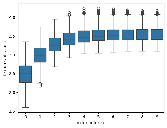
Finally, we provide a helper function to compute “spatial correspondence” - spatial_correspondence(), that is, the average expression distance at increasing spatial distance, as originally proposed by NovoSpaRc [Nitzan et al., 2019].
If a strong spatial correspondence is observed (as in this case) it can be useful to add weight to the spatial coordinates by increasing the alpha value.
df = mp.spatial_correspondence(max_dist=400)
sns.boxplot(x="index_interval", y="features_distance", data=df)
<Axes: xlabel='index_interval', ylabel='features_distance'>