Cell transitions

In this example, we show how to use moscot.plotting.cell_transition().

See also

• See Pull/push distributions on how to plot push-forward and pull-back distributions.

• See Sankey diagram on how to plot the Sankey diagram.

Imports and data loading

import warnings

warnings.simplefilter(action="ignore", category=FutureWarning)

import moscot.plotting as mtp
from moscot import datasets
from moscot.problems.time import TemporalProblem

Load the hspc() dataset.

adata = datasets.hspc()
adata

AnnData object with n_obs × n_vars = 4000 × 2000
    obs: 'day', 'donor', 'cell_type', 'technology', 'n_genes'
    var: 'n_cells', 'highly_variable', 'means', 'dispersions', 'dispersions_norm'
    uns: 'cell_type_colors', 'hvg', 'neighbors', 'neighbors_atac', 'pca', 'umap'
    obsm: 'X_lsi', 'X_pca', 'X_umap_ATAC', 'X_umap_GEX', 'peaks_tfidf'
    varm: 'PCs'
    obsp: 'connectivities', 'distances', 'neighbors_atac_connectivities', 'neighbors_atac_distances'

Prepare and solve the problem

First, we need to prepare and solve the problem. Here, we set the threshold parameter to a relatively high value to speed up convergence at the cost of lower quality solution.

tp = TemporalProblem(adata).prepare(time_key="day").solve(epsilon=1e-2, threshold=1e-2)

INFO     Ordering Index(['4c45fb900fbb', 'c462df3e03b5', '27b9aa554758', '9a0cbad09594',                           
                '98b88fc30c58', '5008d863224a', '904d6bcfd520', '5287a74337a0',                                    
                '862d6d6e4e49', '288e38fb37aa',                                                                    
                ...                                                                                                
                '038518e366a9', '809ba84a9cbb', '4264c55de7d0', 'a7097007fbea',                                    
                '1381ec6cb466', '946cf349f84e', 'da6baa1b0624', 'ba7d40e15f3d',                                    
                '69451694ec4c', '193992d571a5'],                                                                   
               dtype='object', name='cell_id', length=4000) in ascending order.                                    
INFO     Computing pca with `n_comps=30` for `xy` using `adata.X`                                                  

INFO     Computing pca with `n_comps=30` for `xy` using `adata.X`                                                  
INFO     Computing pca with `n_comps=30` for `xy` using `adata.X`                                                  
INFO     Solving `3` problems                                                                                      
INFO     Solving problem BirthDeathProblem[stage='prepared', shape=(766, 1235)].                                   

No GPU/TPU found, falling back to CPU. (Set TF_CPP_MIN_LOG_LEVEL=0 and rerun for more info.)

INFO     Solving problem BirthDeathProblem[stage='prepared', shape=(1235, 1201)].                                  
INFO     Solving problem BirthDeathProblem[stage='prepared', shape=(1201, 798)].                                   

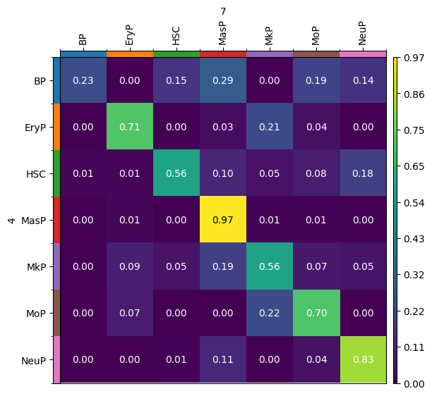
As for all plotting functionalities in moscot, we first call the cell_transition() method of the problem class, which stores the results of the computation in the AnnData instance. Let us assume we want to plot the cell transition between time point 4–7. Moreover, we want the rows and columns of our transition matrix to represent cell types. In general, we can aggregate by any categorical column in obs via the source_groups parameter and the target_groups parameter, respectively. Moreover, we are interested in descendants as opposed to ancestors, which is why we choose forward = True.

cell_transition = tp.cell_transition(
    source=4,
    target=7,
    source_groups="cell_type",
    target_groups="cell_type",
    forward=True,
)

Plot cell transitions

cell_transition is a data frame containing all the information needed, we now want to nicely visualize the result with moscot.plotting.cell_transition(). Therefore, we can either pass the AnnData instance or the problem instance. Depending on the size of our transition matrix, we might want to adapt the dpi and the fontsize parameters. If we don’t want to plot the values of the transition, e.g., because the transition matrix is very large, we can simply set the annotation = False.

mtp.cell_transition(tp, dpi=100, fontsize=10)

By default, the result of the moscot.plotting.cell_transition() method of a problem instance is saved in adata.uns['moscot_results']['cell_transition']['cell_transition'] and overrides this element every time the method is called. To prevent this, we can specify the parameter key_added, which we will do to store the results of the following use case.

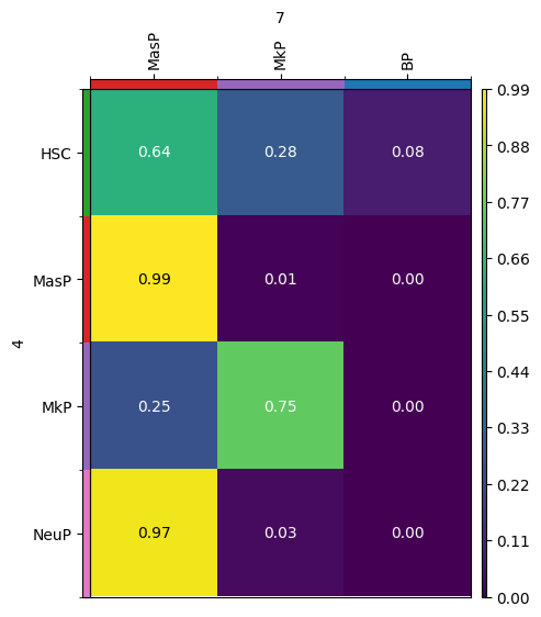
We can also visualize transitions of only a subset of categories of an obs column by passing a dictionary for source_groups or target_groups. Moreover, passing a dictionary also allows to specify the order of the source_groups and target_groups, respectively.

new_key = "subset_cell_transition"
tp.cell_transition(
    source=4,
    target=7,
    source_groups={"cell_type": ["HSC", "MasP", "MkP", "NeuP"]},
    target_groups={"cell_type": ["MasP", "MkP", "BP"]},
    forward=True,
    key_added=new_key,
)
mtp.cell_transition(tp, dpi=100, fontsize=10, key=new_key)