Sankey diagram¶

This example shows how to use moscot.plotting.sankey().

Imports and data loading¶

import moscot.plotting as mtp
from moscot import datasets
from moscot.problems.time import TemporalProblem

Load the hspc() dataset.

adata = datasets.hspc()
adata

AnnData object with n_obs × n_vars = 4000 × 2000
    obs: 'day', 'donor', 'cell_type', 'technology', 'n_genes'
    var: 'n_cells', 'highly_variable', 'means', 'dispersions', 'dispersions_norm'
    uns: 'cell_type_colors', 'hvg', 'neighbors', 'neighbors_atac', 'pca', 'umap'
    obsm: 'X_lsi', 'X_pca', 'X_umap_ATAC', 'X_umap_GEX', 'peaks_tfidf'
    varm: 'PCs'
    obsp: 'connectivities', 'distances', 'neighbors_atac_connectivities', 'neighbors_atac_distances'

Prepare and solve the problem¶

First, we need to prepare and solve the problem. Here, we set the threshold parameter to a relative high value to speed up convergence at the cost of lower quality.

tp = TemporalProblem(adata).prepare(time_key="day").solve(epsilon=1e-2, threshold=1e-2)

INFO     Computing pca with `n_comps=30` for `xy` using `adata.X`                                                  
INFO     Computing pca with `n_comps=30` for `xy` using `adata.X`                                                  
INFO     Computing pca with `n_comps=30` for `xy` using `adata.X`                                                  
INFO     Solving problem BirthDeathProblem[stage='prepared', shape=(766, 1235)].                                   
INFO     Solving problem BirthDeathProblem[stage='prepared', shape=(1235, 1201)].                                  
INFO     Solving problem BirthDeathProblem[stage='prepared', shape=(1201, 798)].                                   

As with all plotting functionalities in moscot, we first call the sankey() method of the problem class, which stores the results of the computation in the AnnData instance. Let us assume we want to plot the Sankey diagram across all time points 2, 3, 4, and 7 . Moreover, we want the Sankey diagram to visualize flows between cell types. In general, we can visualize the flow defined by any categorical column in obs via the source_groups and the target_groups parameters, respectively.

In this example, we are interested in descendants as opposed to ancestors, which is why we choose forward = True. The information required to plot the Sankey diagram is provided in transition matrices, which are saved to adata.uns['moscot_results']['sankey'] by default. Here, we are only interested in the visualization.

tp.sankey(
    source=2,
    target=7,
    source_groups="cell_type",
    target_groups="cell_type",
    forward=True,
)

Plot the Sankey diagram¶

Having called the sankey() method of the problem instance, we now pass the result to the moscot.plotting.sankey(). Therefore, we can either pass the AnnData instance or the problem instance. We can set the size of the figure via dpi and set a title via title.

mtp.sankey(tp, dpi=100, title="Cell type evolution over time")

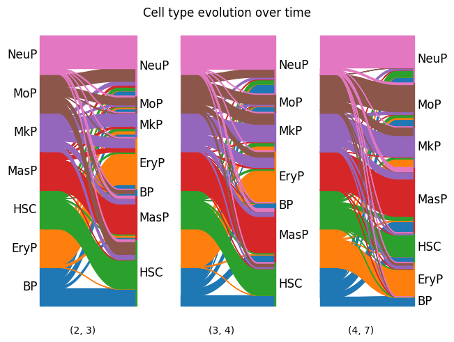
../../../_images/2cde6dfbbd16323ea7c0c13d1377f4ae331391589e5c7c90a521748def3e0fce.png

By default, the result of the moscot.plotting.sankey() is saved in adata.uns['moscot_results']['sankey']['sankey'] and overrides this element every time the method is called. To prevent this, we can specify the parameter key_added, as shown below.

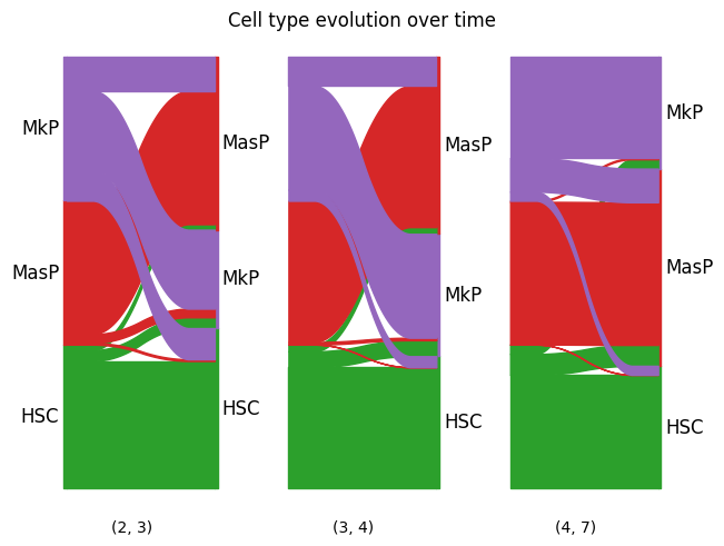
We can also visualize flows of only a subset of categories by passing a dict for source_groups or target_groups. The key should correspond to a value in a categorical obs column and the values to the subset of interest.

new_key = "subset_sankey"
tp.sankey(
    source=2,
    target=7,
    source_groups={"cell_type": ["HSC", "MasP", "MkP"]},
    target_groups={"cell_type": ["HSC", "MasP", "MkP"]},
    forward=True,
    key_added=new_key,
)
mtp.sankey(tp, dpi=100, title="Cell type evolution over time", key=new_key)

../../../_images/2a6aff90610a6deb842debaa704b6a5fc01de02ec5f8a3e57e17c3c10ba01f0c.png