Translating multiomics single-cell data

In this tutorial, we showcase the use of the TranslationProblem, as outlined in [Demetci et al., 2022], to integrate different modalities of single-cell data. In particular, we compute a mapping to translate chromatin accessibility (ATAC) and gene expression (RNA).

The method

The TranslationProblem uses Fused Gromov-Wasserstein (FGW) [Vayer et al., 2020], a type of Optimal Transport (OT), for computing cell-to-cell correspondence probabilities between multiomics single-cell data. As input data, we consider a Latent Semantic Indexing (LSI) embedding for the ATAC data and a Principal Component Analysis (PCA) embedding of the RNA. Since these distinct feature spaces are not directly comparable, we employ a quadratic Gromov-Wasserstein (GW) [Nitzan et al., 2019, Peyré et al., 2016] term that compares pairwise ATAC and RNA cells and seeks to preserve some local geometry between similar cells. Additionally, we may include a linear Wasserstein (W) term that contains a scVI integration of the gene expression raw counts of the RNA and the gene activity raw counts of the ATAC data. Leaving out the linear term makes this a pure GW problem.

Additionally, we use entropic regularization [Cuturi, 2013] to speed up computations and to improve the statistical properties of the solution [Peyré et al., 2019]. In the objective function, we compare \(N\) source (here ATAC) to \(M\) target (here RNA) cells. We use the following definitions:

• \(\varepsilon\): weight given to entropic regularitation. Larger values will lead to more “blurred” couplings.

• \(\alpha\): weight given to GW (distinct features) vs. W (joint features) terms.

Preliminaries

import warnings

import moscot.plotting as mtp
from moscot import datasets
from moscot.problems.cross_modality import TranslationProblem

import numpy as np
import pandas as pd
import scipy
from sklearn import preprocessing as pp

import matplotlib.pyplot as plt

import anndata as ad
import scanpy as sc

warnings.simplefilter("ignore", UserWarning)
warnings.simplefilter("ignore", FutureWarning)

Define utility functions

We will use the average FOSCTTM (fraction of samples closer to the true match) measure implemented below for evaluation (metric used in [Demetci et al., 2022]). This metric measures the alignment between two domains by computing the average fraction of samples that are closer to their true match than a fixed sample, where a perfect alignment results in a FOSCTTM value of zero.

def foscttm(
    x: np.ndarray,
    y: np.ndarray,
) -> float:
    d = scipy.spatial.distance_matrix(x, y)
    foscttm_x = (d < np.expand_dims(np.diag(d), axis=1)).mean(axis=1)
    foscttm_y = (d < np.expand_dims(np.diag(d), axis=0)).mean(axis=0)
    fracs = []
    for i in range(len(foscttm_x)):
        fracs.append((foscttm_x[i] + foscttm_y[i]) / 2)
    return np.mean(fracs).round(4)

Dataset description

This dataset contains preprocessed bone marrow mononuclear cell data from the Open Problems - Multimodal Single-Cell Integration* NeurIPS competition 2021.

Within the bone_marrow() dataset, we store two AnnData objects for the Site 1, Donor 1 ATAC and RNA data. The dataset includes the LSI and PCA embedding of ATAC and RNA respectively, as well as the scVI integration of gene expression and gene activity.

Data loading

We download the bone_marrow() data (approx. 43MiB).

adata_atac = datasets.bone_marrow(rna=False)
adata_rna = datasets.bone_marrow(rna=True)
adata_atac, adata_rna

(AnnData object with n_obs × n_vars = 6224 × 8000
     obs: 'ATAC_nCount_peaks', 'ATAC_nucleosome_signal', 'cell_type', 'batch'
     uns: 'cell_type_colors', 'neighbors'
     obsm: 'ATAC_lsi_full', 'ATAC_lsi_red', 'X_umap', 'geneactivity_scvi'
     layers: 'counts'
     obsp: 'connectivities', 'distances',
 AnnData object with n_obs × n_vars = 6224 × 2000
     obs: 'GEX_n_counts', 'GEX_n_genes', 'cell_type', 'batch'
     uns: 'cell_type_colors', 'neighbors'
     obsm: 'GEX_X_pca', 'X_umap', 'geneactivity_scvi'
     layers: 'counts'
     obsp: 'connectivities', 'distances')

Preprocessing

We perform a L2-normalization of the ATAC data using sklearn.preprocessing.normalize to scale the samples to have unit norm. This is useful, since we quantify the similarity of pair of samples.

adata_atac.obsm["ATAC_lsi_l2_norm"] = pp.normalize(
    adata_atac.obsm["ATAC_lsi_red"], norm="l2"
)

Visualization

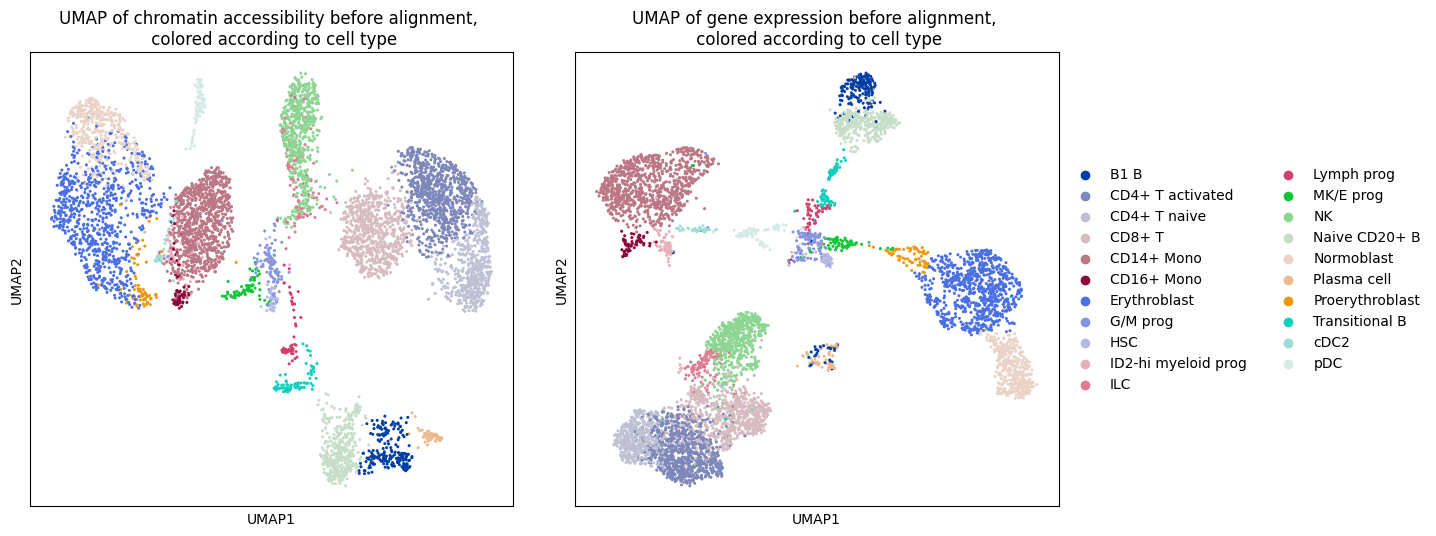
Let’s take a look at the ATAC and RNA data by plotting a UMAP of the respective domain before the alignment, colored according to cell type.

fig, (ax1, ax2) = plt.subplots(1, 2, figsize=(15, 6))
sc.pl.umap(adata_atac, color="cell_type", ax=ax1, show=False)
ax1.legend().remove()
ax1.set_title(
    "UMAP of chromatin accessibility before alignment, \n colored according to cell type"
)
sc.pl.umap(adata_rna, color="cell_type", ax=ax2, show=False)
ax2.set_title(
    "UMAP of gene expression before alignment, \n colored according to cell type"
)
plt.tight_layout(pad=3.0)
plt.show()

Prepare the TranslationProblem

We need to initialize the TranslationProblem by passing the source and target AnnData objects. After initialization, we need to prepare() the problem. In this particular case, we need to pay attention to 3 parameters:

• src_attr: specifies the attribute in AnnData that contains the source distribution. In our case it refers to the key in obsm that stores the ATAC LSI embedding.

• tgt_attr: specifies the attribute in AnnData that contains the target distribution. In our case it refers to the key in obsm that stores the RNA PCA embedding.

• joint_attr[optional]: specifies a joint attribute over a common feature space to incorporate a linear term into the quadratic optimization problem. Initially, we consider the pure Gromov-Wasserstein setting and subsequently explore the fused problem.

tp = TranslationProblem(adata_src=adata_atac, adata_tgt=adata_rna)
tp = tp.prepare(src_attr="ATAC_lsi_l2_norm", tgt_attr="GEX_X_pca")

Solve the TranslationProblem

In fused quadratic problems, the alpha parameter defines the convex combination between the quadratic and linear terms. By default, alpha = 1, that is, we only consider the quadratic problem, ignoring the joint_attr. We choose a small value for epsilon to obtain a sparse transport map.

tp = tp.solve(alpha=1.0, epsilon=1e-3)

INFO     Solving `1` problems                                                                                      
INFO     Solving problem OTProblem[stage='prepared', shape=(6224, 6224)].                                          

Translate the TranslationProblem

We can now project one domain onto the other. The boolean parameter forward determines the direction of the barycentric projection. In our case, we project the source distribution AnnData (ATAC) onto the target distribution AnnData (RNA), therefore we use forward = True. The function translate() returns the translated object in the target space (or source space respectively).

translated = tp.translate(source="src", target="tgt", forward=True)

Analyzing the translation

We will use the average FOSCTTM metric implemented above to analyze the alignment performance.

print(
    "Average FOSCTTM score of translating ATAC onto RNA: ",
    foscttm(adata_rna.obsm["GEX_X_pca"], translated),
)

Average FOSCTTM score of translating ATAC onto RNA:  0.4686

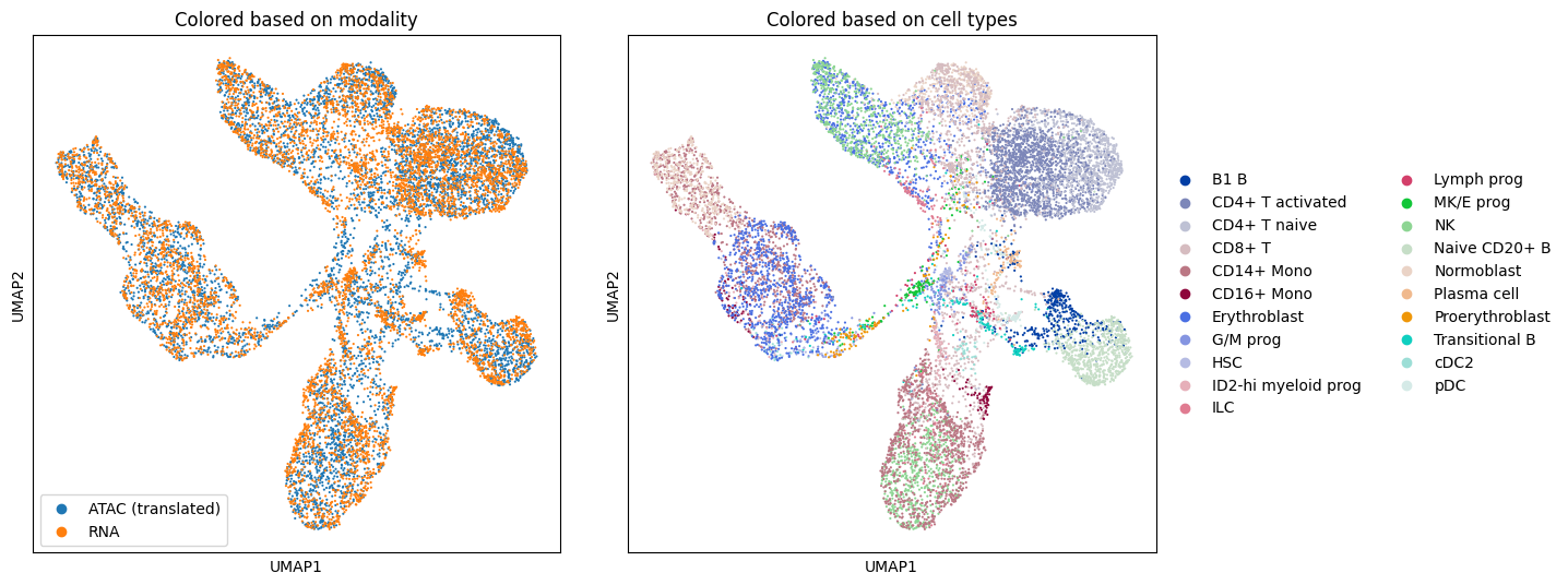
For the sake of visualization, we concatenate the translated chromatin accessibility points mapped to the gene expression PCA domain to the original gene expression PCA data. Then we plot a UMAP of the concatenated data in the gene expression domain, colored according to the original domain and cell type.

adata = sc.concat(
    [adata_atac, adata_rna],
    join="outer",
    label="batch",
    keys=["ATAC (translated)", "RNA"],
)
adata.obsm["X_translated_1"] = np.concatenate(
    (translated, adata_rna.obsm["GEX_X_pca"]), axis=0
)
sc.pp.neighbors(adata, use_rep="X_translated_1")
sc.tl.umap(adata)

fig, (ax1, ax2) = plt.subplots(1, 2, figsize=(15, 6))
sc.pl.umap(adata, color=["batch"], ax=ax1, show=False)
ax1.legend()
ax1.set_title("Colored based on modality")
sc.pl.umap(adata, color=["cell_type"], ax=ax2, show=False)
ax2.set_title("Colored based on cell types")
plt.tight_layout(pad=3.0)
plt.show()

Extend the TranslationProblem to the fused setting

We proceed to extend the TranslationProblem to incorporate the fused setting. In this regard, we aim to evaluate the potential benefits of augmenting the quadratic problem with a linear term. Therefore, we prepare() a new problem, by employing a scVI integration of the gene activity data in the joint_attr. Then, we solve() the resulting problem, with alpha=0.7 and epsilon=.5e-2.

ftp = TranslationProblem(adata_src=adata_atac, adata_tgt=adata_rna)
ftp = ftp.prepare(
    src_attr="ATAC_lsi_l2_norm", tgt_attr="GEX_X_pca", joint_attr="geneactivity_scvi"
)
ftp = ftp.solve(epsilon=0.5e-2, alpha=0.7)
translated_fused = ftp.translate(source="src", target="tgt", forward=True)
print(
    "Average FOSCTTM score for translating ATAC onto RNA: ",
    foscttm(adata_rna.obsm["GEX_X_pca"], translated_fused),
)

INFO     Solving `1` problems                                                                                      
INFO     Solving problem OTProblem[stage='prepared', shape=(6224, 6224)].                                          
Average FOSCTTM score for translating ATAC onto RNA:  0.0524

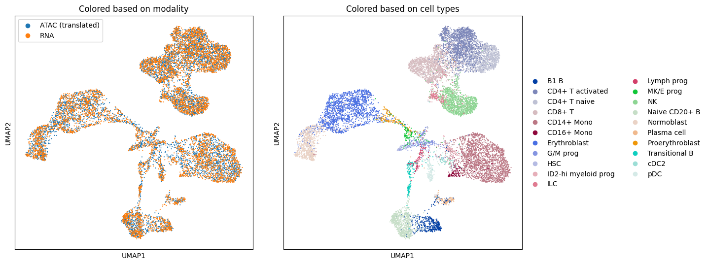
The experimental results demonstrate a significant improvement in the fused setting when compared to the pure Gromov-Wasserstein case.

Visualize translation

adata.obsm["X_translated_2"] = np.concatenate(
    (translated_fused, adata_rna.obsm["GEX_X_pca"]), axis=0
)
sc.pp.neighbors(adata, use_rep="X_translated_2")
sc.tl.umap(adata)

fig, (ax1, ax2) = plt.subplots(1, 2, figsize=(15, 6))
sc.pl.umap(adata, color=["batch"], ax=ax1, show=False)
ax1.legend()
ax1.set_title("Colored based on modality")
sc.pl.umap(adata, color=["cell_type"], ax=ax2, show=False)
ax2.set_title("Colored based on cell types")
plt.tight_layout(pad=3.0)
plt.show()

Analyzing cell type transitions

The cell type transition matrix provides a mapping of cell types from one modality to another and can be used to examine the correspondence between cell types across different datasets. The resulting matrix illustrates which cell types are mapped where thereby enabling further downstream analyses. We order the annotations explicitly by providing a dictionary for source_groups and target_groups.

order = adata_atac.obs["cell_type"].cat.categories

cell_transition = ftp.cell_transition(
    source="src",
    target="tgt",
    source_groups={"cell_type": order},
    target_groups={"cell_type": order},
    forward=True,
    key_added="ftp_transitions",
)

mtp.cell_transition(ftp, figsize=(5, 5), uns_key="ftp_transitions")

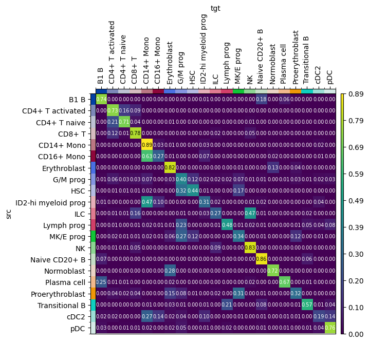
The rows sum up to 1, as for each cell type in a certain row, the columns indicate where the cells are translated to. The TranslationProblem fails to distinguish between ILC and NK cells as only 27/100 ILC cells are mapped correctly while 47/100 ILC cells are mapped to NK cells. In contrast, 89% of CD14+ Mono cells are correctly mapped to CD14+ Mono cells.