Spatiotemporal trajectory of mouse organogenesis

In this tutorial, we showcase the use of SpatioTemporalProblem, which combines gene expression with spatial information, to analyze the spatiotemporal trajectory in mouse organogenesis.

Note

We recommend running this tutorial on a GPU.

See also

• See Analyzing HSPCs with the TemporalProblem on how to link cells across time points without spatial information.

Mapping cells across time incorporating spatial information

The advent of spatially-resolved single-cell datasets of developmental systems enables the characterization of cellular differentiation in space and time. We can utilize OT to learn a matching between cellular states within spatiotemporal datasets by defining a FGW-type problem [Vayer et al., 2020]. In this setup we incorporate similarities at gene expression across time points (W term) and physical distances within time point (GW term).

Additionally, we use entropic regularization [Cuturi, 2013] to speed up computations and to improve the statistical properties of the solution [Peyré et al., 2019]. In the objective function, we compare \(N\) early to \(M\) late cells. We use the following definitions:

• \(P \in \mathbb{R}^{N \times M}\): coupling matrix we seek to learn; it probabilistically relates early to late cells.

• \(C\): cost matrix between early and late cells; it quantifies how “expensive” it is to move along the phenotypic landscape. Typically, it represents Euclidean distance in a gene expression-based latent space like PCA or scVI [Lopez et al., 2018].

• \(C^X\) and \(C^Y\): cost matrices among early and late cells, respectively. These quantify physical distances between the cells. Typically using the l2 distance over obsm['spatial'].

• \(\varepsilon\): weight given to entropic regularitation. Larger values will lead to more “blurred” couplings.

• \(\alpha\): weight given to OT (gene expression) vs. GW (spatial information) terms.

Preliminaries

import warnings

import moscot as mt
import moscot.plotting as mtp
from moscot import datasets
from moscot.problems.spatiotemporal import SpatioTemporalProblem

import numpy as np

import matplotlib.pyplot as plt

import scanpy as sc
import squidpy as sq

warnings.simplefilter("ignore", UserWarning)

Dataset description

The mosta() dataset is a subset of the spatiotemporal transcriptomics atlas of mouse organogenesis [Chen et al., 2022].

The AnnData object includes read-outs at three time points with embryo sections E9.5_E2S1, E10_E2S1, and E11.5_E1S2. The data was preprocessed by normalizing and log-transforming the counts.

adata = datasets.mosta()
adata

AnnData object with n_obs × n_vars = 54134 × 2000
    obs: 'annotation', 'timepoint', 'n_genes_by_counts', 'log1p_n_genes_by_counts', 'total_counts', 'log1p_total_counts', 'pct_counts_in_top_50_genes', 'pct_counts_in_top_100_genes', 'pct_counts_in_top_200_genes', 'pct_counts_in_top_500_genes', 'time', 'n_genes', 'total_counts_mt', 'pct_counts_mt', 'Heart_mapping', 'Heart_annotation'
    var: 'n_cells_by_counts', 'mean_counts', 'log1p_mean_counts', 'pct_dropout_by_counts', 'total_counts', 'log1p_total_counts', 'n_cells', 'mt', 'highly_variable', 'highly_variable_rank', 'means', 'variances', 'variances_norm', 'highly_variable_nbatches'
    uns: 'Heart_annotation_colors', 'annotation_colors', 'hvg', 'moscot_results'
    obsm: 'spatial'
    layers: 'count'

Visualise the data

We consider the cell type annotations in spatial coordinates.

library_ids = list(adata.obs["timepoint"].cat.categories)
sq.pl.spatial_scatter(
    adata,
    color="annotation",
    frameon=False,
    shape=None,
    library_key="timepoint",
    library_id=library_ids,
    title=library_ids,
    figsize=(10, 10),
    size=[50, 5, 5],
    legend_fontsize=15,
)

Prepare the SpatioTemporalProblem

We start by initializing a problem

stp = SpatioTemporalProblem(adata)

We can adapt the marginals of the OT problem. By default, marginals are chosen to be uniform. This means that, even if each cell in the early time point has multiple possible descendants in the later time point, the proportions of the descendants sum up to “the mass of one cell”. In developing systems we know that some cells might proliferate more than others. We can account for this by adapting the marginals based on proliferation and apoptosis markers with score_genes_for_marginals().

See also

• See Handling marginals on how to pass custom marginals.

stp = stp.score_genes_for_marginals(
    gene_set_proliferation="mouse", gene_set_apoptosis="mouse"
)

WARNING: genes are not in var_names and ignored: ['Anln', 'Anp32e', 'Atad2', 'Aurka', 'Aurkb', 'Birc5', 'Blm', 'Brip1', 'Bub1', 'Casp8ap2', 'Cbx5', 'Ccnb2', 'Ccne2', 'Cdc20', 'Cdc25c', 'Cdc45', 'Cdc6', 'Cdca2', 'Cdca3', 'Cdca7', 'Cdca8', 'Cdk1', 'Cenpa', 'Cenpe', 'Cenpf', 'Chaf1b', 'Ckap2', 'Ckap2l', 'Ckap5', 'Cks1b', 'Cks2', 'Clspn', 'Ctcf', 'Dlgap5', 'Dscc1', 'Dtl', 'E2f8', 'Ect2', 'Exo1', 'Fam64a', 'Fen1', 'G2e3', 'Gas2l3', 'Gins2', 'Gmnn', 'Gtse1', 'Hells', 'Hjurp', 'Hjurp', 'Hmgb2', 'Hmmr', 'Hn1', 'Kif11', 'Kif20b', 'Kif23', 'Kif2c', 'Lbr', 'Mcm2', 'Mcm4', 'Mcm5', 'Mcm6', 'Mki67', 'Mlf1ip', 'Msh2', 'Nasp', 'Ncapd2', 'Ndc80', 'Nek2', 'Nuf2', 'Nusap1', 'Pcna', 'Pola1', 'Pold3', 'Prim1', 'Psrc1', 'Rad51', 'Rad51ap1', 'Rangap1', 'Rfc2', 'Rpa2', 'Rrm1', 'Rrm2', 'Slbp', 'Smc4', 'Tacc3', 'Tipin', 'Tmpo', 'Top2a', 'Tpx2', 'Ttk', 'Tubb4b', 'Tyms', 'Ubr7', 'Uhrf1', 'Ung', 'Usp1', 'Wdr76']
WARNING: genes are not in var_names and ignored: ['Abat', 'Abcc5', 'Abhd4', 'Acvr1b', 'Ada', 'Adck3', 'Aen', 'Ak1', 'Alox8', 'Ankra2', 'Apaf1', 'App', 'Atf3', 'Baiap2', 'Bak1', 'Bax', 'Blcap', 'Bmp2', 'Btg1', 'Casp1', 'Ccnd3', 'Ccng1', 'Ccnk', 'Ccp110', 'Cd81', 'Cd82', 'Cdkn2a', 'Cdkn2aip', 'Cdkn2b', 'Cebpa', 'Cgrrf1', 'Csrnp2', 'Ctsd', 'Ctsf', 'Cyfip2', 'Dcxr', 'Ddb2', 'Ddit3', 'Ddit4', 'Def6', 'Dgka', 'Dnttip2', 'Dram1', 'Ei24', 'Epha2', 'Ephx1', 'Eps8l2', 'Ercc5', 'F2r', 'Fam162a', 'Fas', 'Fbxw7', 'Fdxr', 'Fos', 'Foxo3', 'Fuca1', 'Gadd45a', 'Gls2', 'Gm2a', 'Gnb2l1', 'Gpx2', 'H2afj', 'Hbegf', 'Hdac3', 'Hexim1', 'Hint1', 'Hist1h1c', 'Hmox1', 'Hras', 'Hspa4l', 'Ier3', 'Ier5', 'Ikbkap', 'Il1a', 'Inhbb', 'Ip6k2', 'Irak1', 'Iscu', 'Itgb4', 'Jag2', 'Jun', 'Kif13b', 'Klf4', 'Klk8', 'Ldhb', 'Lrmp', 'Mapkapk3', 'Mdm2', 'Mknk2', 'Mxd1', 'Mxd4', 'Ndrg1', 'Ninj1', 'Nol8', 'Notch1', 'Nudt15', 'Nupr1', 'Osgin1', 'Pcna', 'Pdgfa', 'Phlda3', 'Plk2', 'Plk3', 'Plxnb2', 'Pmm1', 'Polh', 'Pom121', 'Ppm1d', 'Ppp1r15a', 'Prkab1', 'Prmt2', 'Procr', 'Ptpn14', 'Ptpre', 'Rab40c', 'Rad51c', 'Rad9a', 'Ralgds', 'Rap2b', 'Rb1', 'Rchy1', 'Retsat', 'Rgs16', 'Rhbdf2', 'Rnf19b', 'Rpl18', 'Rps12', 'Rps27l', 'Rrp8', 'Rxra', 'S100a10', 'S100a4', 'Sat1', 'Sdc1', 'Sec61a1', 'Serpinb5', 'Sertad3', 'Sesn1', 'Slc19a2', 'Slc35d1', 'Slc3a2', 'Socs1', 'Sp1', 'Sphk1', 'St14', 'Steap3', 'Stom', 'Tap1', 'Tax1bp3', 'Tcn2', 'Tgfa', 'Tgfb1', 'Tm4sf1', 'Tm7sf3', 'Tob1', 'Tpd52l1', 'Tprkb', 'Traf4', 'Trafd1', 'Triap1', 'Trib3', 'Trp53', 'Trp63', 'Tsc22d1', 'Tspyl2', 'Txnip', 'Upp1', 'Vamp8', 'Vdr', 'Vwa5a', 'Wrap73', 'Wwp1', 'Xpc', 'Zbtb16', 'Zfp365', 'Zfp36l1', 'Zmat3']

To prepare the problem we need to pass some information:

• time_key: defines the obs column for the temporal information.

• spatial_key: defines the obsm where the spatial coordinates are saved used to claculate \(C^X\) and \(C^Y\).

• joint_attr: defines based on which (latent) space we compute the distances for the W problem, \(C\). Here, we do not use a precomputed embedding but hence pass None and use a callback.

• callback: states which computation should be run on X to get the joint cost.

See also

• See Custom cost matrices on how to pass precomputed cost matrices.

• See Subset policy on how to choose pairs of time points between which to compute OT maps.

stp = stp.prepare(
    time_key="time",
    spatial_key="spatial",
    joint_attr=None,
    callback="local-pca",
)

INFO     Computing pca with `n_comps=30` for `xy` using `adata.X`                                                  
INFO     Computing pca with `n_comps=30` for `xy` using `adata.X`                                                  

Solve the SpatioTemporalProblem

As the data is large, we use low-rank optimal transport to decrease the computational complexity [Scetbon et al., 2021].

To solve the problem we pass the following arguments, alpha (in \((0, 1]\)), which defines the influence of the spatial coordinates as opposed to the single-cell data. epsilon, the entropy parameter, and initializer='rank2' to improve the speed of convergence.

See also

• See Linear problems (advanced) on how to modify low-rank parameters.

• See Quadratic problems (advanced) for an advanced example on how to solve quadratic problems.

stp = stp.solve(alpha=0.5, epsilon=1e-3, rank=500, initializer="rank2")

INFO     Solving `2` problems                                                                                      
INFO     Solving problem BirthDeathProblem[stage='prepared', shape=(5870, 18292)].                                 
INFO     Solving problem BirthDeathProblem[stage='prepared', shape=(18292, 29972)].                                

Cell transitions

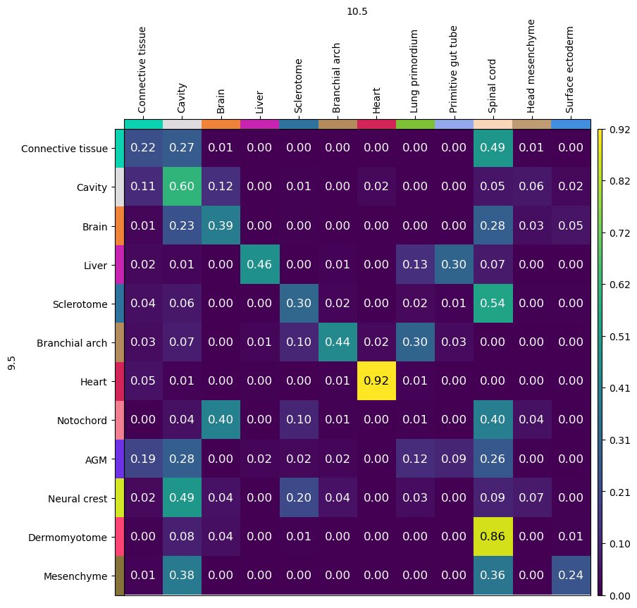
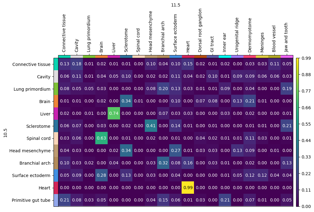
We can now analyze which cell types are mapped to which cell type across time using the cell_transition() method. As different time points have different cell types, it is not straightforward to assess the mapping. To improve the visualization, we order the annotations such that in the upper left we have the same cell types.

celltypes_source_1 = adata[adata.obs["time"] == 9.5].obs["annotation"].cat.categories
celltypes_target_1 = adata[adata.obs["time"] == 10.5].obs["annotation"].cat.categories
celltypes_intersection_1 = list(
    set(celltypes_source_1).intersection(celltypes_target_1)
)
source_ordered_1 = celltypes_intersection_1 + list(
    set(celltypes_source_1) - set(celltypes_target_1)
)
target_ordered_1 = celltypes_intersection_1 + list(
    set(celltypes_target_1) - set(celltypes_source_1)
)

stp.cell_transition(
    source=9.5,
    target=10.5,
    source_groups={"annotation": source_ordered_1},
    target_groups={"annotation": target_ordered_1},
    forward=True,
)
mtp.cell_transition(stp, fontsize=12, figsize=(7, 7))

Most of the cell types seem to map to themselves, such as the Heart cells. Moreover, we can see that many cells are mapped to Cavity, which is to be expected.

celltypes_source_2 = adata[adata.obs["time"] == 10.5].obs["annotation"].cat.categories
celltypes_target_2 = adata[adata.obs["time"] == 11.5].obs["annotation"].cat.categories
celltypes_intersection_2 = list(
    set(celltypes_source_2).intersection(celltypes_target_2)
)
source_ordered_2 = celltypes_intersection_2 + list(
    set(celltypes_source_2) - set(celltypes_target_2)
)
target_ordered_2 = celltypes_intersection_2 + list(
    set(celltypes_target_2) - set(celltypes_source_2)
)

stp.cell_transition(
    source=10.5,
    target=11.5,
    source_groups={"annotation": source_ordered_2},
    target_groups={"annotation": target_ordered_2},
    forward=True,
)
mpl.cell_transition(stp, fontsize=10, figsize=(8, 8))

Pushing cells across space and time

Next, we can visualize the predicted spatial destination of the cells using the push() method. Below we focus on the Heart cells.

for (start, end), prob in stp.problems.items():
    stp.push(
        source=start,
        target=end,
        data="annotation",
        subset="Heart",
        key_added="Heart_mapping",
    )

In the first column, we plot the spatial locations of the heart cells at E10.5. In the second row, we show the Heart cells projected onto the the spatial coordinates at E11.5.

library_ids = ["E10.5", "E11.5"]

sq.pl.spatial_scatter(
    adata,
    color=["Heart_mapping", "Heart_annotation"],
    frameon=False,
    shape=None,
    library_key="timepoint",
    library_id=library_ids,
    cmap="viridis_r",
    figsize=(10, 10),
    size=[20, 10],
    legend_fontsize=15,
)